[논문 리뷰] SDEs: Score-based generative modeling with stochastic differential equations

[논문]

• Score-based generative modeling with stochastic differential equations
• NeurIPS 2021
• Citations: 6,517
• [https://arxiv.org/abs/2011.13456]

 

• 해당 논문 보기 전 참고하면 좋은 post
• Score-based model 리뷰

[개념 설명] Score-based Model

[개념 설명] Score-based Model

 

• NCSN 논문 리뷰

[논문 리뷰] NCSN: Generative modeling by estimating gradients of the data distribution

[논문 리뷰] NCSN: Generative modeling by estimating gradients of the data distribution

 

---

Abstract

• Generative modeling: creating data from noise

 

[Contributions]

• SDE
  • Slowly injecting noise를 통해 complex data dist → known prior dist.
  • Reverse-time SDE
    • time-dependent gradient field of the perturbed data dist에만 depend
      • ⇒ NN을 통해 these scores를 estimate 가능 & numerical SDE solvers를 통해 sampling

 

• Predictor-corrector framework 도입
  • evolution of the discretized reverse-time SDE에서 error를 correct함

 

• Probability flow ODE
  • SDE와 동일한 dist.에서 sampling ⇒ equivalent 증명
  • exact likelihood computation & improved sampling efficiency

 

• New way to solve inverse problems with score-based models
  • Using a single unconditional score-based model without re-training

 

• CIFAR-10의 uncond generation - SOTA
• Competitive likelihood
• score-based generative model에서 처음으로 1024x1024 high fidelity image 생성

 

1. Introduction

• Score matching with Langevin dynamics (SMLD)
  • 각 noise scale에서 score 추정
  • Langevin dynamics를 이용하여 sampling
• Denoising diffusion probabilistic modeling (DDPM)
  • 각 step의 noise corruption을 reverse하기 위해 sequence of prob. models 학습
  • ⇒ Continuous state spaces, DDPM은 각 noise scale에서 denoising을 반복하면서 암묵적으로 score 계산을 예측하게 됨

 

⇒ two model clases를 score-based generative models로 부름

⇒ new sampling methods & further extend the capabilities - SDEs

 

[SDEs]

• Diffusion process을 사용하여 Continuum of dist. 고려
  • data → random noise & prescribed SDE (no trainable parameters)

 

• Reverse process
  • random noise → generated data
  • Reverse-time SDE ⇒ forward SDE를 통해 derive
  • estimated scores with time-dependent NN을 통해 approximate
  • 

 

2. Background

[SMLD]

• $p_\sigma(\tilde x|x)$: perturbation kernel
  •  

    

  • $\sigma_{min}=\sigma_1<...<\sigma_N=\sigma_{max}$

• $s_\theta(x,\sigma)$ ⇒ weighted sum of denoising score matching objectives를 통해 학습
  • $s_\theta(\tilde x,\sigma_i)$, $\nabla_{\tilde x}$ - Not $x$
  • 

 

• optimal score-based model $s_{\theta^*}(x,\sigma) \approx\nabla_xlogp_\sigma(x)$, almost everywhere for $\sigma\in{\sigma_i}_{i=1}^N$

 

• Langevin MCMC sampling for each $p_{\sigma_i}(x)$ sequentially

  • 

    
     
  • $z_i^m\sim N(0,I)$
  • $i=N,N-1, ...,1$
  • $x^0_N\sim N(0, \sigma^2_{max}I)$, $x^0_i=x^M_{i+1}$
  • $M$→ $\infty$ & $\epsilon_i$ → $0$ for all i ⇒ $x_1^M\sim p_{\sigma_{min}}(x)\approx p_{data}(x)$ under some regularity conditions
    • ⇒ $i$는 각 $\sigma_i$에 depent한 $s_\theta$를 통해 첫번째 dt 구한 뒤, Langevin을 통해 update

 

[DDPM]

• positive noise scales $0<\beta_1,...<\beta_N<1$ ⇒ pre-described
• discrete Markov chain ⇒ $p(x_i|x_{i-1})=N(x_i;\sqrt{1-\beta_i}x_{i-1},\beta_iI)$
• $p_{\alpha_i}(x_i|x_0)=N(x_i;\sqrt{\alpha_i}x_0, (1-\alpha_i)I)$, $\alpha_i=\Pi_{j=1}^i(1-\beta_j)$

 

• Similar to SMLD
  • 

• Variational Markov chain in reverse direction

  • 

     
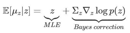
  • Tweedie's Formula 이용
    • exponential family dist.에서 sample이 있을 때 true mean 추정 방법
      • ⇒ $z\sim N(z;\mu_z, \Sigma_z)$, sample 1개
    • MLE의 bias를 score ft를 통해 보정   

      • 

        
             
    • 
    • ⇒ score ft 학습 = noise의 반대 방향(denoising) 학습 with time scaling factor

 

• re-weighted variant of the evidence lower bound (ELBO)
• 

• Ancestral sampling - From the graphical model $\Pi_{i=1}^Np_\theta(x_{i-1}|x_i)$⇒ SMLD와 다르게 each step에서 한번의 sampling 후 다음 step으로 넘어감
• 

 

[Objective]

• SMLD
• 

• DDPM
• 

⇒ $L_{simple}$을 SMLD $L$와 비슷하게 작성

 

• SMLD와 유사하게 weighted sum of denoising score matching mojectives
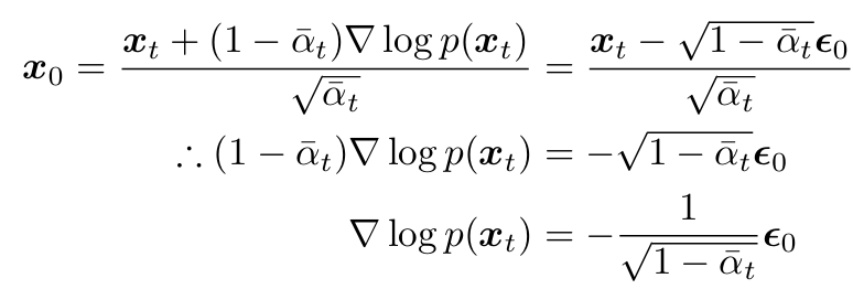
• $s_{\theta^*}(\tilde x,i)\approx \nabla_xlogp_{\alpha_i}(x)$
• weight - perturbation kernels과 관련

  • 

  • ⇒ $\nabla_xlogp_{\sigma_i}(\tilde x|x)=-\frac{\tilde x-x}{\sigma_i^2}$ & $\nabla_xlogp_{\alpha_i}(\tilde x|x)=-\frac{\tilde x-x}{(1-\alpha_i)^2}$

 

3. Score-Based generative modeling with SDEs

• Generalize multiple noise scales ⇒ infinite number of noise scales

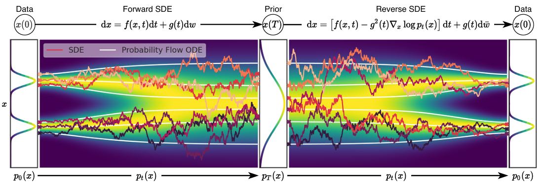
3.1 Perturbing data with SDEs

• Goal: construct a diffusion process ${x(t)}^T_{t=0}$
  • $x(0)\sim p_0$, i.i.d samples dataset ⇒ data dist.
  • $x(T)\sim p_T$, tractable form ⇒ prior dist.

 

• Ito SDE의 solution ⇒ Diffusion process

  • 

     
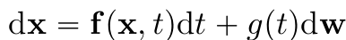
  • $g(t)$: diffusion coefficient, Scalar & Not depend on $x$
  • Globally Lipschitz조건 만족시 SDE는 unique strong solution 가짐
    • $|f(x_1,t) - f(x_2,t)|$≤$K|x_1-x_2|$, $|g(x_1)-g(x_2)|$≤$K|x_1-x_2|$
  • data dist. → fixed prior dist.로 diffuse될 수 있게 SDE design

 

• $p_t(x)$: $x(t)$의 probability density
• $p_{st}(x(t)|x(s))$: $x(s)$
  →$x(t)$의 transition kernel, $0$≤$s$<$t$≤$T$
• $p_T$: unstructured prior dist. ⇒ no information of $p_0$

 

3.2 Generating samples by reversing time SDE

• $x(T)\sim p_T$의 samples에서 시작하여 $x(0)\sim p_0$의 samples을 obtain
• Reverse-time SDE

  • 

  • $\bar w$: $T$→$0$의 standard wiener process
  • $dt$: negative timestep

 

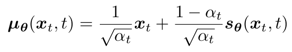
3.3 Estimating scores for the SDE

• Score matching

  • 

  • time-dependent score-based model $s_\theta(x,t)$를 train
  • $t\sim U(0,T)$
  • $s_{\theta^*}(x,t)=\nabla_xlogp_t(x)$, for almost all $x$ and $t$
  • SMLD, DDPM과 비슷하게 positive weighting ft $\lambda(t)$사용
  • 

 

• Transition kernel $p_{0t}(x(t)|x(0))$
  • f(., t)가 affine하다면 transition kernel은 항상 Gaussian dist. ⇒ closed-forms으로 구할 수 있음

 

3.4 Examples: VE, VP SDEs and beyond

[SMLD]

• each perturbation kernel: $p_{\sigma_i}(x|x_0)\sim N(x, \sigma_i)$
• Noise 점진적으로 추가 ⇒ Markov chain
  • $p(x_i|x_{i-1})\sim N(x_{i-1}, (\sigma^2_i-\sigma^2_{i-1})I)$
  • 
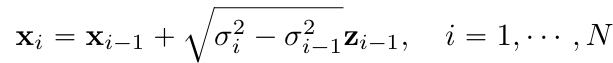
  • $z_{i-1}\sim N(0,I)$, $\sigma_0=0$
  • $N$→$\infty$ ⇒ ${\sigma_i}^N_{i=1}$→$\sigma(t)$ & $z_i$→$z(t)$ & ${x_i}^N_{i=1}$→${x(t)}^1_{t=0}$, t$\in[0,1]$

 

• Rewrite markov chain
  • Let $x(i/N)=x_i,$ $\sigma(i/N)=\sigma_1,$ $z(i/N)=z_i$, $i=1,...,N$
  • $\Delta(t)=1/N$, $t\in{0, 1/N, ...,(N-1)/N}$
  • 

• If $\Delta t$→0, $w(t+\Delta t)-w(t)=dw(t)\sim N(0,\Delta tI)$
  • $dw=\sqrt{\Delta t}z(t)$

 

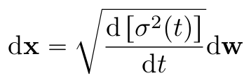
• SMLD는 Variance Explonding (VE) SDEs
  • when t→$\infty$, variance exploding
  • 

 

[DDPM]

• each perturbation kernel: $p_{\alpha_i}(x|x_0)\sim N(\alpha_ix_0, (1-\alpha_i)I)$
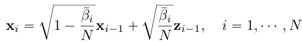
• Discrete markov chain
  •  

    

  • $z_{i-1}\sim N(0,I)$
  • $N$→$\infty$, ${\bar{\beta_i}=N\beta_i}^N_{i=1}$

 

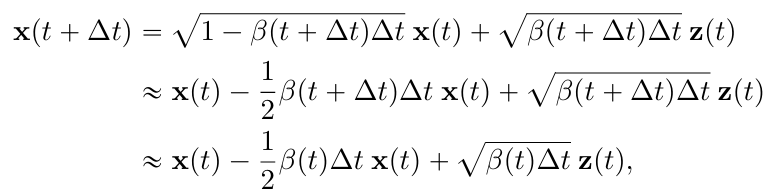
• Rewrite markov chain

  • 

  • $N$→$\infty$ ⇒ ${\bar{\beta_i}}^N_{i=1}$→$\beta(t)$ & $t\in[0,1]$
  • Let $\beta(i/N)=\bar{\beta_i}$, $x(1/N)=x_i$, $z(i/N)=z_i$
  • $\Delta t=1/N$, $t\in{0, 1/N, ...,(N-1)/N}$
  • 

 

• DDPM은 Variance Preserving (VP) SDE
  • when t→$\infty$, fixed variance of one
  • 

 

[sub-VP SDE]

• likelihoods에 perform particularly ⇒ 저자 propose

  • 

  • 모든 intermediate time step에서 variance가 VP SDE보다 작거나 같음
  • intermediate step에서도 안정적인 분산 유지 ⇒ 과도한 noise 추가 X

 

 

⇒ VE, VP, sub-VP SDEs는 affine drift coefficients를 가짐

• $p_{0t}(x(t)|x(0))$은 Gaussian & closed-forms이므로 efficient 학습 가능

 

4. Solving thet reverse SDE

4.1 General-purpose numerical SDE solvers

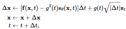
• Numerical sovlers - SDEs로부터 approx. trajectories 제공
  • Euler-Maruyama, stochastic Runge-Kutta methods
    • stochastic dynamics를 discretizations하는 방법들
  • reverse-time SDE를 통해 sampling 진행

 

• Ancestral sampling - DDPM 방법
  • reverse-time VP SDE의 special discretization
  • 

 

⇒ SDEs에서 non-trivial하기에, reverse diffusion samplers propose

• forward SDEs와 동일한 방식으로 reverse SDE를 discretization
  • ⇒ 쉽게 derive & discretization과정에서 수치적 불안정성 문제 해결

 

 

• Reverse diffusion이 SMLD & DDPM에서 better performance 보임
  • Data: CIFAR-10
• Ancestral sampling for SMLD - Appendix F
  • $p(x_i|x_{i-1})\sim N(x_{i-1}, (\sigma^2_i-\sigma^2_{i-1})I)$ ⇒ Markcov chain 후 DDPM과 동일 방법
  • 

 

4.2 Predictor-corrector samplers

• generic SDEs와 달리, solutions 향상을 위해 additional information 사용
  • $s_{\theta^*}(x,t)\approx\nabla_xlogp_t(x)$ ⇒ score-based MCMC approaches 사용가능
    • $p_t$에서 직접 sampling 가능
  • numerical SDE solver의 solution을 correct해줌

 

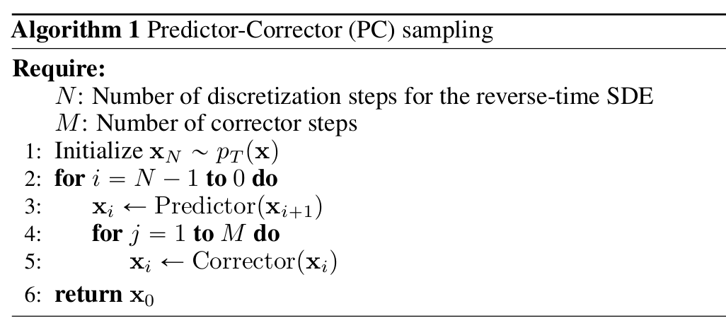
• numerical SDE sovler - next time step의 sample estimate 계산 ⇒ “predictor”
• score-based MCMC approach - estimated sample의 marginal dist.를 correct ⇒ “corrector”
  • ⇒ Predictor-Corrector (PC) samplers
  • ⇒ Predictor-Corrector methods와 유사 (Allgower & Georg, 2012)

 

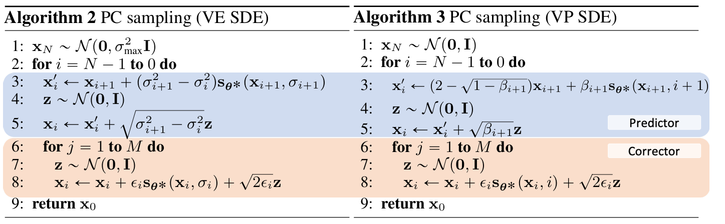
• PC samplers - SMLD & DDPM의 generalization
  • SMLD - predictor = identity ft.(sigma변경, 분포이동) & corrector = Langevin dynamics
  • DDPM - predictor = Ancestral sampling & corrector = identity

 

 

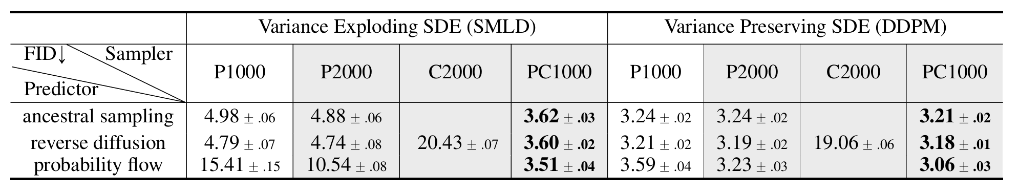
• Reverse diffusion >>> Ancestral sampling
• C2000 << P2000, PC1000 (same computation)
• P1000 < PC1000 (one corrector step for each predictor step)
• P2000 < PC1000

⇒ 즉 predictor보다 corrector를 추가하는 것이 better performance

 

4.3 Probability flow and connection to neural ODEs

• 모든 SDEs는 same marginal dist. ${p_t(x)}^T_{t=0}$를 가지는 deterministic process 존재
  •  

    

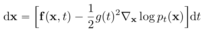
  • deterministic process는 ODE를 만족 → $s_\theta(x)\approx\nabla_xlogp_t(x)$ with NN
    • ⇒ Neural ODE

 

[Exact likelihood computation]

• Neural ODEs를 활용하면 ODE와 instantaneuous change of variavles formular를 통해 likelihood 계산 가능
• uniformly dequantized data의 log-likelihood 계산
  • Dequantized data - data를 continuous dist.로 처리할 수 있도록 만듦
    • ex) Uniform Dequantization: $x_{dequan} = x_{orig}+u$, $u\sim N(0,1)$
  • DDPM($L/L_{simple}$)은 discrete data의 ELBO values

 

[Manipulating latent representations]

• $x(0)$→$x(T)$→$x(0)$ 복원 가능
• Neural ODEs 및 Normalizing Flows와 마찬가지로, latent representations 조작할 수 있음
• interpolation, temperature scaling과 같은 image editing을 통해 조작할 수 있음

 

[Uniquely identifiable encoding]

• most current invertible models과 다르게 uniquely identifiable한 encoding을 가짐
  • $x(0)$는 고유한 $x(T)$를 가짐
  • forward SDE는 no trainable parameters를 가지기 때문 & dw term 없음

 

[Efficient sampling]

• black-box ODE solver사용하면 high quality samples을 얻을 수 있고, efficiency를 위해 accuracy를 trade-off할 수 있음
  • sampling 속도 up

 

4.4 Architecture improvements

• VE SDEs의 optimal architecutre: NCSN++
• VP SDEs의 optimal architecutre: DDPM++
• cont - Ep (7)인 continuous objective 사용하여 train ⇒ 성능 up
• deep - network depth 2배
• VE SDE의 NCSN++ high quality samples 제공
• VP SDE의 DDPM++ high likelihood 제공

 

5. Controllable generation

• $p_t(y|x(t))$ known ⇒ $p_0(x(0)|y)$로 부터 sampling 가능

 

• Conditional reverse-time SDE

  • 

  • 이를 이용하여 large family of inverse problems with score-based generative models 해결
    • given estimate of $\nabla_xlogp_t(y|x)$

 

• Appendix I.4 - auxiliary models 학습없이 해당 estimate obtain하는 방법 소개

 

• Class-conditional generation
  • time-dependent classifier $p_t(y|x(t))$ 학습

 

• Imputation - conditional sampling의 special case
  • incomplete data point y가 주어졌을 때, 누락된 부분 imputation하여 복원
  • $\Omega(y)$는 y의 잘 알려진 부분
  • Colorization - imputation의 special case
    • 흑백 & coloar image의 관계를 orthogonal linear transform을 통해 decoupling
    • transformed space에서 imputation을 진행하여 colorization perform